Advertisement
Q-learning doesn’t require a map of the environment or a set strategy. That’s part of what makes it interesting—and tricky. In Part 1, we looked at the basics: what Q-learning is, the concept of Q-values, the role of rewards, and the update rule. This part goes further. Now, we’ll focus on how Q-learning plays out in real tasks, what affects its learning, and how it performs in different environments. This shift from theory to application is where it starts to feel less abstract and more like a tool that can solve real problems.
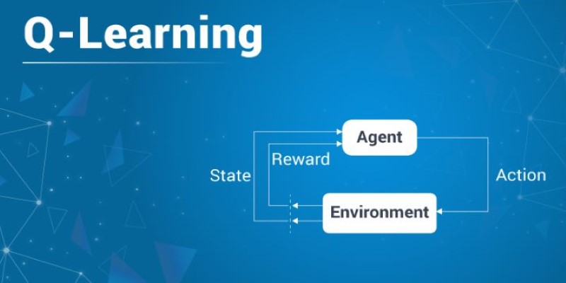
At the centre of Q-learning is the agent-environment loop. The agent begins without any real knowledge. It selects an action in a given state, sees the result (reward and new state), and updates its Q-table. Over time, it learns which actions lead to better rewards by repeating this cycle.

A key factor is how the agent chooses actions. If it always selects what looks best, it might miss better options. If it picks randomly, learning becomes inefficient. This is known as the exploration vs exploitation tradeoff. A common method to manage this is the ε-greedy strategy. With a small probability ε, the agent picks a random action; the rest of the time, it goes with the highest Q-value. This allows early exploration and more focused actions later.
The Q-table stores expected rewards for each state-action pair. Early on, all values may be zero. However, after many rounds of feedback, the table reflects smarter decisions. Each update helps the agent respond better next time it's in a similar situation.
Three main settings shape how learning unfolds: the learning rate (α), the discount factor (γ), and the exploration rate (ε).
The learning rate decides how much new information overrides old. A small α means slower updates and more memory of past actions. A large α updates Q-values quickly but can make learning unstable. Choosing a balanced α is important for steady improvement.
The discount factor controls how much the agent values future rewards. A γ near 0 makes the agent short-sighted, focusing on immediate payoffs. A γ close to 1 makes it value long-term outcomes more. Many tasks work well with γ between 0.8 and 0.99.
ε defines how often the agent explores. Early in training, it should explore often. Later, as the Q-table becomes more reliable, it should explore less. A common tactic is to slowly reduce ε over time. This approach encourages early discovery and later stability.
Given enough time and proper tuning, Q-values begin to settle—a process called convergence. If every state-action pair is visited often enough and the learning rate shrinks with time, Q-learning can converge to the best strategy. In real scenarios, full convergence is rare, but agents often reach a reliable level of performance.
In small, well-defined spaces, Q-learning works well. For instance, a robot in a 5x5 grid can learn to reach a goal by trying different paths and adjusting its Q-table after each step. Over time, the Q-values guide it through the best route.
As environments grow more complex, the limitations of Q-learning show. In tasks with large or continuous spaces, storing every state-action pair in a table becomes impractical. This is where function approximation helps. Instead of a table, a model—often a neural network—estimates Q-values. This version is called Deep Q-Learning (DQN). It allows learning from rich inputs like images and makes it possible to generalize across similar situations.
Sparse rewards can also be a challenge. When feedback only comes at the end of a long task, it's hard to tell which actions helped. One solution is reward shaping, where the agent gets smaller rewards for making progress. For example, the robot might earn points for moving closer to a goal, not just reaching it.
Another concern is overfitting. The agent might perform well in one environment but fail when things change slightly. To address this, the training environment can be varied, or randomness can be introduced. This helps the agent learn flexible strategies that work in more than one situation.
Q-learning is well-suited to problems where the environment is stable, the number of states is limited, and feedback is available frequently enough to guide learning. Since it doesn't require knowledge of how the environment works, it's useful for problems where that information is unavailable or too complex to model.
That said, there are limits. Standard Q-learning doesn't scale well to large environments. Deep Q-Learning helps, but it comes with added complexity. Q-learning also assumes that the agent can observe the full state. In many tasks, such as real-world robotics or games, only part of the environment is visible. In such cases, more advanced methods are needed.
Delayed rewards also make learning harder. When the payoff for a good decision comes much later, the agent struggles to assign credit. Eligibility traces offer a partial fix by keeping a short memory of recent actions, spreading the reward backwards over time.
Despite its boundaries, Q-learning remains a foundational method in reinforcement learning. It’s often used as a base for other techniques and helps build intuition for how trial-and-error learning can work.
Q-learning is a simple idea with surprising depth. It helps agents learn to make decisions by interacting with the world without being told what to do. This second part focused on how Q-learning works in practice, how settings like the learning rate and exploration rate influence outcomes, and how it performs in both small tasks and more complex ones. We also looked at its limitations and the ways people work around them. For anyone looking to understand how machines can learn from experience, Q-learning is a good place to start—and still widely used today.
Advertisement
Curious about Meta-RL? Learn how meta-reinforcement learning helps data science systems adapt faster, use fewer samples, and evolve smarter—without retraining from scratch every time

How Hugging Face for Education makes AI accessible through user-friendly machine learning models, helping students and teachers explore natural language processing in AI education

Discover lesser-known Pandas functions that can improve your data manipulation skills in 2025, from query() for cleaner filtering to explode() for flattening lists in columns
Learn how Apache Oozie coordinates Hadoop jobs with XML workflows, time-based triggers, and clean orchestration. Ideal for production-ready data pipelines and complex ETL chains

Should credit risk models focus on pure accuracy or human clarity? Explore why Explainable AI is vital in financial decisions, balancing trust, regulation, and performance in credit modeling

How a course launch community event can boost engagement, create meaningful interaction, and shape a stronger learning experience before the course even starts

Curious why developers are switching from Solidity to Vyper? Learn how Vyper simplifies smart contract development by focusing on safety, predictability, and auditability—plus how to set it up locally

Is your team using AI tools you don’t know about? Shadow AI is growing inside companies fast—learn how to manage it without stifling innovation or exposing your data
Curious how stacking boosts model performance? Learn how diverse algorithms work together in layered combinations to improve accuracy—and why stacking goes beyond typical ensemble methods

Curious what’s really shaping AI and tech today? See how DataHour captures real tools, honest lessons, and practical insights from the frontlines of modern data work—fast, clear, and worth your time
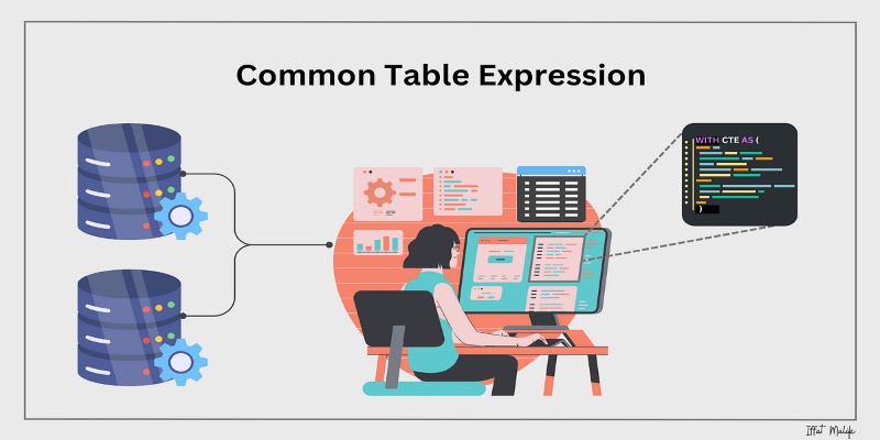
Learn what a Common Table Expression (CTE) is, why it improves SQL query readability and reusability, and how to use it effectively—including recursive CTEs for hierarchical data

Explore how Google Cloud Platform (GCP) powers scalable, efficient, and secure applications in 2025. Learn why developers choose GCP for data analytics, app development, and cloud infrastructure